Parse Charts in PDFs and Analyze with Pandas

This tutorial shows how to parse a PDF with specialized chart parsing enabled, extract table data from a page that contains a chart, and run basic data science with pandas. We use the same 2024 Executive Summary PDF as in Parse a PDF & Interpret Outputs; the third page includes a chart that Parse can turn into structured data.

1. Setup

Set your API key as an environment variable so the SDKs pick it up automatically:

export LLAMA_CLOUD_API_KEY="llx-..."

Install the SDK and construct a client. This example analyzes the parsed table with pandas, so the Python tab also installs it.

Python

pip install "llama-cloud>=2.8" pandas

from llama_cloud import LlamaCloud

client = LlamaCloud()  # reads LLAMA_CLOUD_API_KEY from the environment

TypeScript

npm install @llamaindex/llama-cloud

import LlamaCloud from '@llamaindex/llama-cloud';
import fs from 'fs';

const client = new LlamaCloud(); // reads LLAMA_CLOUD_API_KEY from the environment

Go

go get github.com/run-llama/llama-parse-go

import llamacloud "github.com/run-llama/llama-parse-go"

client := llamacloud.NewClient() // reads LLAMA_CLOUD_API_KEY from the environment

Java

implementation("ai.llamaindex:llama-cloud:1.3.0")

import ai.llamaindex.llamacloud.client.LlamaCloudClient;
import ai.llamaindex.llamacloud.client.okhttp.LlamaCloudOkHttpClient;

// reads LLAMA_CLOUD_API_KEY from the environment
LlamaCloudClient client = LlamaCloudOkHttpClient.fromEnv();

CLI

go install github.com/run-llama/llama-parse-cli/cmd/llp@latest

llp reads LLAMA_CLOUD_API_KEY from the environment (or pass --api-key).

The analysis in later steps uses pandas (Python only) — every language can parse the chart PDF and pull out the table; the DataFrame work is Python-specific.

2. Parse with Specialized Chart Parsing

Specialized chart parsing tells Parse to extract chart and graph data with higher fidelity. Enable it via processing_options and request the items view so you get structured tables (and figures) per page.

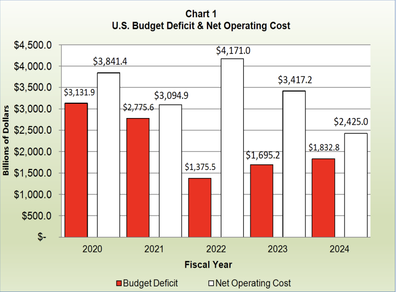
We parse the same executive summary PDF and request items so we can pull tables from page 3, which contains the following chart:

In Python and TypeScript, expand is passed to the parse call. In Go, Java, and the CLI, expand is a query parameter on the result fetch, so those create the job, poll until it reaches a terminal status, then request the items view.

Python

# Upload the file
file = client.files.create(file="./executive-summary-2024.pdf", purpose="parse")

# Parse with specialized chart parsing, and request the items view
result = client.parsing.parse(
    file_id=file.id,
    tier="agentic_plus",
    version="latest",
    processing_options={"specialized_chart_parsing": "agentic_plus"},
    expand=["items"],
)

TypeScript

// Upload the file
const file = await client.files.create({
  file: fs.createReadStream('./executive-summary-2024.pdf'),
  purpose: 'parse',
});

// Parse with specialized chart parsing, and request the items view
const result = await client.parsing.parse({
  file_id: file.id,
  tier: 'agentic_plus',
  version: 'latest',
  processing_options: { specialized_chart_parsing: 'agentic_plus' },
  expand: ['items'],
});

Go

// Upload the file
f, err := os.Open("./executive-summary-2024.pdf")
if err != nil {
  log.Fatal(err)
}
defer f.Close()

file, err := client.Files.New(ctx, llamacloud.FileNewParams{File: f, Purpose: "parse"})
if err != nil {
  log.Fatal(err)
}

// Parse with specialized chart parsing (expand is a GET parameter in Go)
job, err := client.Parsing.New(ctx, llamacloud.ParsingNewParams{
  FileID:  llamacloud.String(file.ID),
  Tier:    llamacloud.ParsingNewParamsTierAgenticPlus,
  Version: llamacloud.ParsingNewParamsVersionLatest,
  ProcessingOptions: llamacloud.ParsingNewParamsProcessingOptions{
    SpecializedChartParsing: "agentic_plus",
  },
})
if err != nil {
  log.Fatal(err)
}

// Poll until the job reaches a terminal status, then request the items view
getParams := llamacloud.ParsingGetParams{Expand: []string{"items"}}
result, err := client.Parsing.Get(ctx, job.ID, getParams)
if err != nil {
  log.Fatal(err)
}
for result.Job.Status != "COMPLETED" && result.Job.Status != "FAILED" && result.Job.Status != "CANCELLED" {
  time.Sleep(2 * time.Second)
  result, err = client.Parsing.Get(ctx, job.ID, getParams)
  if err != nil {
    log.Fatal(err)
  }
}
if result.Job.Status != "COMPLETED" {
  log.Fatalf("parse ended as %s", result.Job.Status)
}

Java

// Upload the file
FileCreateResponse file = client.files().create(FileCreateParams.builder()
        .file(Paths.get("./executive-summary-2024.pdf"))
        .purpose("parse")
        .build());

// Parse with specialized chart parsing (expand is a query parameter in Java)
ParsingCreateResponse job = client.parsing().create(ParsingCreateParams.builder()
        .fileId(file.id())
        .tier(ParsingCreateParams.Tier.AGENTIC_PLUS)
        .version(ParsingCreateParams.Version.LATEST)
        .processingOptions(ParsingCreateParams.ProcessingOptions.builder()
                .specializedChartParsing(
                        ParsingCreateParams.ProcessingOptions.SpecializedChartParsing.AGENTIC_PLUS)
                .build())
        .build());

// Poll until the job reaches a terminal status, then request the items view
ParsingGetParams getParams = ParsingGetParams.builder()
        .jobId(job.id())
        .addExpand("items")
        .build();

ParsingGetResponse result = client.parsing().get(getParams);
while (!result.job().status().equals(ParsingGetResponse.Job.Status.COMPLETED)
        && !result.job().status().equals(ParsingGetResponse.Job.Status.FAILED)
        && !result.job().status().equals(ParsingGetResponse.Job.Status.CANCELLED)) {
    Thread.sleep(2000);
    result = client.parsing().get(getParams);
}
if (!result.job().status().equals(ParsingGetResponse.Job.Status.COMPLETED)) {
    throw new RuntimeException("parse ended as " + result.job().status());
}

CLI

# Upload the file
FILE_ID=$(llp files create \
  --file ./executive-summary-2024.pdf \
  --purpose parse | jq -r '.id')

# Parse with specialized chart parsing
JOB_ID=$(llp parsing create \
  --file-id "$FILE_ID" \
  --tier agentic_plus \
  --version latest \
  --processing-options.specialized-chart-parsing agentic_plus \
  | jq -r '.id')

# Poll until the job reaches a terminal status
while true; do
  STATUS=$(llp parsing get --job-id "$JOB_ID" | jq -r '.job.status')
  case "$STATUS" in COMPLETED|FAILED|CANCELLED) break ;; esac
  sleep 2
done

3. Get Table Data from Page 3

The third page of the PDF (index 2 in the items tree) contains a chart. With chart parsing, Parse often represents the chart’s data as a table in the items tree. We collect the first table on that page and use its rows for the analysis.

Python

page_three = result.items.pages[2]  # third page (0-indexed)

tables = [item for item in page_three.items if getattr(item, "type", None) == "table"]
if not tables:
    raise ValueError("No table found on page 3. Try the agentic_plus tier.")

rows = tables[0].rows
print(f"Chart table has {len(rows)} rows")

TypeScript

const pageThree = result.items.pages[2]; // third page (0-indexed)

let rows;
for (const item of pageThree.items) {
  if ('type' in item && item.type === 'table' && 'rows' in item) {
    rows = item.rows;
    break;
  }
}
if (!rows) {
  throw new Error('No table found on page 3. Try the agentic_plus tier.');
}
console.log(`Chart table has ${rows.length} rows`);

Go

page := result.Items.Pages[2] // third page (0-indexed)

var rows [][]*llamacloud.TableItemRowUnion
for _, item := range page.Items {
  if item.Type == "table" {
    rows = item.Rows
    break
  }
}
if rows == nil {
  log.Fatal("No table found on page 3. Try the agentic_plus tier.")
}
fmt.Printf("Chart table has %d rows\n", len(rows))

Java

ParsingGetResponse.Items.Page page = result.items().get().pages().get(2); // third page (0-indexed)
if (!page.isStructuredResult()) {
    throw new RuntimeException("No table found on page 3. Try the agentic_plus tier.");
}
ParsingGetResponse.Items.Page.StructuredResultPage pageThree = page.asStructuredResult();

var rows = pageThree.items().stream()
        .filter(ParsingGetResponse.Items.Page.StructuredResultPage.Item::isTable)
        .findFirst()
        .orElseThrow(() -> new RuntimeException("No table found on page 3. Try the agentic_plus tier."))
        .asTable()
        .rows();

System.out.println("Chart table has " + rows.size() + " rows");

CLI

# Pull the rows of the first table on page 3 (index 2)
llp parsing get --job-id "$JOB_ID" --expand items \
  | jq '.items.pages[2].items | map(select(.type == "table"))[0].rows'

4. Load the Fiscal-Year Chart into Pandas

The analysis below uses Python + pandas. The chart on this page is a grouped bar chart showing Budget Deficit and Net Operating Cost (both in billions of dollars) for fiscal years 2020–2024. We turn its table into a clean time-series DataFrame:

import pandas as pd

# First row as column names, rest as data
header = rows[0]
df = pd.DataFrame(rows[1:], columns=header)

money_cols = [
    "Budget Deficit (Billions of Dollars)",
    "Net Operating Cost (Billions of Dollars)",
]

df["Fiscal Year"] = df["Fiscal Year"].astype(int)

print("DataFrame:")
print(df)

DataFrame:
   Fiscal Year Budget Deficit (Billions of Dollars)  \
0         2020                             $3,131.9
1         2021                             $2,775.6
2         2022                             $1,375.5
3         2023                             $1,695.2
4         2024                             $1,832.8

  Net Operating Cost (Billions of Dollars)
0                                 $3,841.4
1                                 $3,094.9
2                                 $4,171.0
3                                 $3,417.2
4                                 $2,425.0

5. Analyze Deficit vs. Net Operating Cost

With the data cleaned, we can reproduce the key relationships described under the chart text.

1. Year-over-year changes in both series

df["Deficit YoY Change"] = df["Budget Deficit (Billions of Dollars)"].diff()
df["Net Operating Cost YoY Change"] = df["Net Operating Cost (Billions of Dollars)"].diff()

print(df[["Fiscal Year",
          "Budget Deficit (Billions of Dollars)",
          "Net Operating Cost (Billions of Dollars)",
          "Deficit YoY Change",
          "Net Operating Cost YoY Change"]])

   Fiscal Year  Budget Deficit (Billions of Dollars)  \
0         2020                                3131.9
1         2021                                2775.6
2         2022                                1375.5
3         2023                                1695.2
4         2024                                1832.8

   Net Operating Cost (Billions of Dollars)  Deficit YoY Change  \
0                                    3841.4                 NaN
1                                    3094.9              -356.3
2                                    4171.0             -1400.1
3                                    3417.2               319.7
4                                    2425.0               137.6

   Net Operating Cost YoY Change
0                            NaN
1                         -746.5
2                         1076.1
3                         -753.8

This highlights, for example, the sharp spike in net operating cost in 2022 and the decline through 2023–2024.

2. Gap between Net Operating Cost and Budget Deficit

df["Gap (Net Operating Cost - Deficit)"] = (
    df["Net Operating Cost (Billions of Dollars)"]
    - df["Budget Deficit (Billions of Dollars)"]
)

print("\nGap between Net Operating Cost and Budget Deficit (billions):")
print(df[["Fiscal Year", "Gap (Net Operating Cost - Deficit)"]])

print("\nYear with largest gap:")
print(df.loc[df["Gap (Net Operating Cost - Deficit)"].idxmax()])

print("\nYear with smallest gap:")
print(df.loc[df["Gap (Net Operating Cost - Deficit)"].idxmin()])

Gap between Net Operating Cost and Budget Deficit (billions):
   Fiscal Year  Gap (Net Operating Cost - Deficit)
0         2020                               709.5
1         2021                               319.3
2         2022                              2795.5
3         2023                              1722.0
4         2024                               592.2

Year with largest gap:
Fiscal Year                                 2022.0
Budget Deficit (Billions of Dollars)        1375.5
Net Operating Cost (Billions of Dollars)    4171.0
Deficit YoY Change                         -1400.1
Net Operating Cost YoY Change               1076.1
Gap (Net Operating Cost - Deficit)          2795.5
Name: 2, dtype: float64

Year with smallest gap:
Fiscal Year                                 2021.0
Budget Deficit (Billions of Dollars)        2775.6
Net Operating Cost (Billions of Dollars)    3094.9
Deficit YoY Change                          -356.3
Net Operating Cost YoY Change               -746.5
Gap (Net Operating Cost - Deficit)           319.3
Name: 1, dtype: float64

This reproduces the narrative that 2022 saw the largest divergence between the two metrics, while by 2024 the gap had narrowed significantly.

3. Quick visualization (optional)

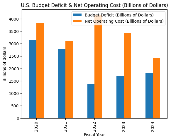
ax = df.plot(
    x="Fiscal Year",
    y=[
        "Budget Deficit (Billions of Dollars)",
        "Net Operating Cost (Billions of Dollars)",
    ],
    kind="bar",
    title="U.S. Budget Deficit & Net Operating Cost (Billions of Dollars)",
)
ax.set_ylabel("Billions of dollars")

This bar chart closely mirrors Chart 1 in the PDF, but now backed by a DataFrame that you can further slice, aggregate, or feed into downstream analytics.

Summary

• Use specialized chart parsing (processing_options.specialized_chart_parsing: "agentic" or "agentic_plus") when your PDF has charts you want as structured data.
• Request items in expand to get per-page tables (and figures).
• Pull table rows from the page that contains the chart (here, page 3), then build a pandas DataFrame from rows and run summaries, plots, or filters as needed.

For more options (e.g. efficient vs agentic), see Specialized Chart Parsing.